Regular and Singular Groups (RS) attempts to calculate the lengths of secret messages hidden in natural images by measuring the noise added by LSB Replacement (LSBR). RS is based on the fact that the LSB values in natural images are not random. The pixels in natural images tend to blend into each other, similar to a gradient. Steganography using LSBR adds noise (artificial randomness) to the image. This noise can be measured. RS is a type of statistical analysis steganalysis.
Let us assume our stego-image is greyscale and is 8 x 8 pixels. The adjacent pixels on each row are divided into groups of n pixels, where n is a factor of the number of bytes in each row. For example, if n = 4, the first group will consist of pixels 0 - 3, the second group will consist of pixels 4 - 7, and so on.
A discrimination function, f, is applied to each group of pixels. The purpose of f is to measure the amount of noise in each group. A simple way to achieve this is to calculate the sum of the absolute differences of the adjacent pixels in each group. For example, using the group (251, 252, 180, 192) gives us 251 − 252 = −1, 252 − 180 = 72, and 180 − 192 = 1. The sum of the absolute differences is 74.
If the pixels in a group have similar values (low amount of noise), f will return a small value. If the pixels have dissimilar values (more noise), f will return a larger value.
There are two additional functions which can be applied to each group. Both of these functions simulate hiding messages of varying lengths in the LSBs. The function F1 replaces LSBs using LSBR, whereas the function F−1 replaces LSBs similar to LSB Matching (LSBM), but does not prevent 0 becoming −1, and 255 becoming 0.
The discrimination function f is also applied to the results of F1 and F−1. This means we use f to calculate (a) the amount of noise for each group of pixels, (b) the amount of noise for each group of pixels after the LSBs have been replaced according to F1, and (c) the amount of noise for each group of pixels after the LSBs have been replaced according to F−1. The results of (a) and (b), and (a) and (c) can be compared to create three new groups:
* Regular groups, R, are the groups where LSB changes increased the amount of noise.
* Singular groups, S, are the groups where LSB changes decreased the amount of noise.
* Unusable groups, U, are the groups where LSB changes neither increased nor decreased the amount of noise. This group can be ignored.
(As an aside, a cover image will typically return more R groups, as both F1 and F−1 are introducing noise. Additionally, the number of R and S groups will be consistent such that RF1 = RF−1 and SF1 = SF−1).
We can plot R and S on a graph using three predefined message lengths:
* p/2 is a hidden message of any length less than 100% embedding. The reason it is p/2 rather than p is because around half the LSBs will already be set to the desired value.
* 50 is a hidden message of 100% embedding.
* 1 − p/2 is a hidden message of 100% embedding, but where all the LSBs had to
be changed.
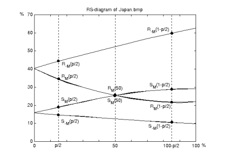
As can be seen in the above image (a diagram showing how the length of the message p embedded in a test image called Japan.bmp affects the number of R and S groups; note the subscripts M and −M can be considered equivalent to F1 and F−1, respectively), plotting the points for the three predefined message lengths for both F1 and F−1 gives us five pairs of R and S groups spread over nine points. These points connect to create four intersecting curves, typically two straight lines and two polynomials. What is important to note here is the above image could be any natural image - there will always be four curves and nine predictable points. For example, if the image contains a hidden message of any length, F−1 will always produce a higher number of R groups compared to F1.
The four curves allow us to find the length of the hidden message p. Using the above image as an example, if we change the x−axis so p/2 becomes 0, and 100 − p/2 becomes 1, the x-coordinate of the intersection point RM(50), SM(50) is a root of the following quadratic equation:
2(d1 + d0)x² + (d−0 − d−1 − d1 − 3d0)x + d0 − d−0 = 0, where
d0 = RM(p/2) − SM(p/2)
d1 = RM(1 − p/2) − SM(1 − p/2)
d−0 = R−M(p/2) − S−M(p/2)
d−1 = R−M(1 − p/2) − S−M(1 − p/2)
We can then calculate p using the absolute value of the root x where p = x/(x − 1/2).
To calculate p for an RGB image, each colour channel is treated like a separate greyscale-like image: one image using all the red bytes, one image using all the green bytes, and one image using all the blue bytes. The output is the estimation of LSB changes for each colour channel.